FRS17 Case Study

by P Barber (April 2010)

(Back)

Introduction

1. The requirements of FRS 17 necessitated the valuation of the Company’s unfunded pension obligations. Under a now obsolete scheme a selected number of people on leaving the Company had been granted a grace-and-favour index-linked pension, which was paid out of Company funds. In recent years the number of pensioners on this scheme has reduced to single digit levels, and annual pension payments amount to some £13,000 in total and a provision of £162,400 has been deemed sufficient to cover the outstanding obligation.

 2. The process for calculating the value of the FRS17 provision has been in place for a number of years. It is based on a table of life-expectance, down-loaded from the web, which differentiates between males and females and provides an expected number of years, based on the age of the pensioner. A segment of the table is shown below:

Life Expectancy
Age	M	F
66	14.32	18.21
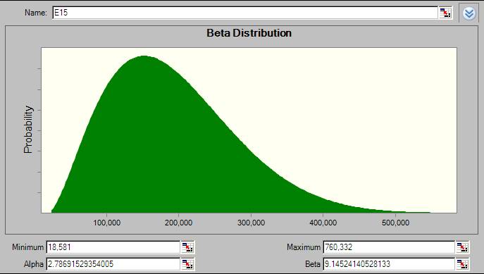
67	13.7	17.48
68	13.09	16.76
69	12.5	16.04
70	11.92	15.35
71	11.35	14.66
"	"	"
99	2.34	2.64
100	2.22	2.48
101	2.11	2.34
102	1.99	2.2
103	1.89	2.06
104	1.78	1.93
"	"	"
115	0.89	0.89
116	0.83	0.83
117	0.77	0.77
118	0.71	0.71
119	0.66	0.66

 3. As can be seen from the table above, a male aged 99 years is expected to live for 2.34 years more, or until he is 101.34 years of age (99 years + 2.34 years). However, should he live until he is 100 then his life expectancy is 2.22 years and he is expected to live until he is 102.22 years of age (100 years + 2.22 years)

 4. It was found that when using a model based on the above assumption that the calculated value of the provision altered little from year to year. This find was at odds with the expectation that:

Closing Provision = Opening Provision – amount expended during the year

 5. An investigation was therefore initiated to devise an alternative model, and it is this model which is presented as a case study.

New Model

 6. The search for am alternative model began on the web, and after some investigation an alternative source of life expectancy data was located at the Office of National Statistics. A segment of the table is shown below:

Interim Life Tables, England
Period expectation of life										Office for National Statistics
Based on data for the years 2006-2008
Age	Males					Females
x	mx	qx	lx	dx	ex	mx	qx	lx	dx	ex
0	0.005393	0.005379	100000.0	537.9	77.74	0.004436	0.004426	100000.0	442.6	81.88
1	0.000402	0.000402	99462.1	40.0	77.16	0.000347	0.000347	99557.4	34.6	81.24
2	0.000237	0.000237	99422.1	23.6	76.19	0.000204	0.000204	99522.9	20.3	80.27
3	0.000165	0.000165	99398.6	16.4	75.20	0.000163	0.000163	99502.6	16.2	79.28
4	0.000138	0.000138	99382.2	13.7	74.22	0.000115	0.000115	99486.4	11.4	78.30
5	0.000135	0.000135	99368.5	13.4	73.23	0.000099	0.000099	99475.0	9.9	77.30
6	0.000106	0.000106	99355.1	10.5	72.24	0.000095	0.000095	99465.1	9.4	76.31
7	0.000102	0.000102	99344.6	10.1	71.24	0.000078	0.000078	99455.7	7.7	75.32
8	0.000126	0.000126	99334.5	12.5	70.25	0.000093	0.000093	99448.0	9.3	74.33
9	0.000120	0.000120	99322.0	11.9	69.26	0.000075	0.000075	99438.7	7.5	73.33
10	0.000104	0.000104	99310.1	10.4	68.27	0.000087	0.000087	99431.2	8.6	72.34
11	0.000115	0.000115	99299.7	11.4	67.28	0.000092	0.000092	99422.6	9.1	71.34
12	0.000118	0.000118	99288.3	11.8	66.28	0.000100	0.000100	99413.5	9.9	70.35
13	0.000157	0.000157	99276.5	15.6	65.29	0.000119	0.000119	99403.6	11.8	69.36

 7. The field indicated in the table are:

m_x – the number of deaths, at the age x (last birthday) in the three year period to which the table relates, divided by the average population at that age over the same period.

q_x – the probability that a person aged x (exactly) will die before reaching age (x +1)

l_x – the number of survivors to (exact) age x per 100,000 live births.

d_x – the number dying between exact age x and (x+1) described similarly to l_x, that is d_x = l_x – l_x+1

e_x – the average life expectancy, that is the average number of years that those aged x (exact) will live beyond x

 8. The new model assumes that a pension is paid in full for each year up to the year of death, and that no payment is made thereafter. Although FRS17 suggests that discounting of the cash-flows should be applied, this is not attempted in this model, as there is no attempt to create a specific cash or deposit fund to cover these payments.

 9. It is assumed that the value of the pension is increased by the rate of inflation. The pension payment is therefore modelled using the incremental equation:

Px+1 = Px (Inflation Factor)

Where:

Px = the pension paid in year x.

Px+1 = pension paid in the year following year x, and

Inflation factor is model using a BetaPERT Distribution, defined (in Oracle Crystal Ball) as follows:

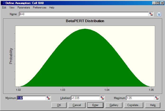
 10. The table below shows a segment of the calculation to determine the pension that might typically be paid to one individual over a period of twelve years. The table shows that a current pension of £7,395 might rise to £10,053 by year 8. In the model the calculation is repeated 10,000 to determine the range of outcomes that might apply. On each iteration and for each year a possible inflation factor is selected at random from the BetaPERT range that has been applied. In this model it has been assumed that the distribution of the inflation factors remains constant through the whole range of the model. However, a different inflation assumption could have been applied to each year, should this have been thought necessary.

	Inflation	Annual
Year	Forecast	Pension
0		7,395
1	1.038726	7,682
2	1.037561	7,970
3	1.046469	8,340
4	1.038355	8,660
5	1.044785	9,048
6	1.031487	9,333
7	1.040164	9,708
8	1.035507	10,053
9	1.038252	10,437
10	1.029655	10,747
11	1.034493	11,117
12	1.032799	11,482

 11. When considering the liability, with regard to a pensioner for a specific year, there are three possibilities:

a) the pensioner survives, in which case the pension plus inflation is paid in that particular year, or

b) the pensioner dies in that year, in which case no payment is made in that particular year, or

c) the pensioner died in a previous year, in which case no payment will be made in that particular year.

12. The probability of death in a particular year is shown in column q_x of the Life Expectancy table, while the probability of survival is given by (1 – q_x).

13. In the example below the process is illustrated with reference to an 89 year-old, female pensioner. Appropriate details from the Life Expectancy table are reproduced below:

Age	Female
x	qx
89	0.122312
90	0.138332
91	0.159600
92	0.178012
93	0.196646
94	0.214254
95	0.234928
96	0.254641
97	0.268735
98	0.298142
99	0.314155
100	0.339337

14. The Life Expectancy table shows that for a female aged 89 years there is a 0.122312 chance of dying before the age of 90 years. However, we are interested in the probability of living, which is (1 – 0.122312 = 0.8777). This probability can be defined by a Yes/No distribution shown below:

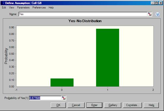
15. During a simulation Oracle Crystal Ball produces a value of 1 on 87.7688% of occasions and a value of zero on 12.2312% of occasions. In the following year (age 90 years) Crystal Ball will produce, at random, a value of zero on 13.8332% of occasions and a value of 1 one 86.1668% of occasions. If a value of zero is selected in a particular year then the values of all subsequent years will also be set to zero. A segment of the simulation, illustrating three iterations, is shown in the Appendix. The result of a full ten-thousand iteration simulation is shown below.

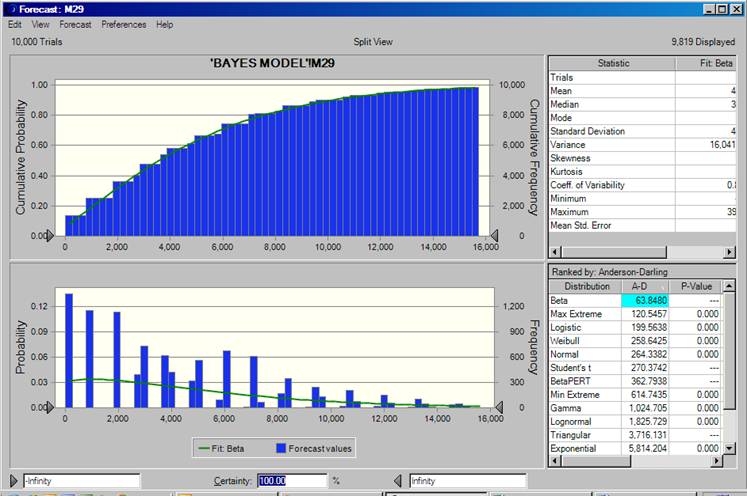
16. Oracle Crystal Ball has suggested that the result of the full simulation is best described by a Beta Distribution. However, with an AD statistic as high as 63.848 the fit is not particularly good. Unfortunately, Oracle Crystal Ball does not provide a P-Value for the Beta Distribution.

17. The results of a simulation for all of the pensioners is shown below.

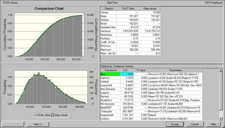
18. With Crystal Ball suggesting that the best fit to the data was a Beta Distribution, with an AD of 0.2053; this option was selected, and is shown in more detail below.

19. The validity of the above result was investigated further (see Appendix 2). It was found that AD statistic could be replicated in an Excel spread sheet, a result which indicated that:

a) The formula for the Beta Distribution available in Excel “BETADIST(x, Alpha, Beta, Minimum, Maximum)” was the same as that employed in Crystal Ball, and

b) That the Anderson Darling statistic was calculated in the same way.

Appendix 1 (page 1)

	In year
	Die = 0	Once	Inflation	Inflated	Possible
Age	Live = 0	Dead = 0	Factor	Payment	Payment
	(a)	(b)	(c)	(d)	(e)
				885
89	1	1	1.0417	922	922
90	1	1	1.0400	959	959
91	1	1	1.0301	988	988
92	1	1	1.0463	1,033	1,033
93	1	1	1.0332	1,068	1,068
94	1	1	1.0323	1,102	1,102
95	1	1	1.0292	1,134	1,134
96	1	1	1.0359	1,175	1,175
97	1	1	1.0234	1,203	1,203
98	1	1	1.0258	1,234	1,234
99	1	1	1.0328	1,274	1,274
100	1	1	1.0325	1,316	1,316
101	1	1	1.0301	1,355	1,355
102	1	1	1.0302	1,396	1,396
103	1	1	1.0363	1,447	1,447
104	1	1	1.0350	1,497	1,497
105	1	1	1.0406	1,558	1,558
106	0	0	1.0331	1,610	0
107	1	0	1.0293	1,657	0
108	1	0	1.0415	1,726	0
			Possible Liability		20,660

a) Column (a) shows that in the first iteration, the options selected result in the pensioner surviving until she is 105 years of age, this is indicated by the unbroken series of ones appearing in column (a)

b) Column (b) monitors the values appearing in column (a) and once a value of zero has occurred ensures that all subsequent values appearing in column (b) are set to zero. “If(Value of (a) = 0, then set to 0, otherwise set to previous value of (b)”

c) Column (c) shows the inflation factors which have been selected.

d) The Inflation Factors from column (c) are used to calculate a possible value for the inflated pension, which appears in column (d). At the start of the simulation the pension is £885, by the time the pensioner reaches 90 years of age the pension is: £885 x 1.0417 x 1.04 = £959

e) The value shown in column (e) shows the value of pension that might be paid. This value is calculated by multiplying column (b) by column (e). For example at 105 years of age 1 x £1,558 = £1,558, while at 106 years of age 0 x £1,610 = 0. The total at the bottom of column (e) indicates that the FRS17 liability, based on all the selected assumptions made during the simulation, might be £20,660

Appendix 1 (page 2)

	In year
	Die = 0	Once	Inflation	Inflated	Possible
Age	Live = 0	Dead = 0	Factor	Payment	Payment
	(a)	(b)	(c)	(d)	(e)
				885
89	1	1	1.0353	916	916
90	1	1	1.0386	952	952
91	1	1	1.0365	986	986
92	1	1	1.0375	1,023	1,023
93	1	1	1.0343	1,058	1,058
94	1	1	1.0320	1,092	1,092
95	1	1	1.0336	1,129	1,129
96	1	1	1.0304	1,163	1,163
97	0	0	1.0341	1,203	0
98	0	0	1.0277	1,236	0
99	1	0	1.0443	1,291	0
100	1	0	1.0373	1,339	0
101	1	0	1.0336	1,384	0
102	1	0	1.0263	1,420	0
103	1	0	1.0301	1,463	0
104	0	0	1.0385	1,520	0
105	1	0	1.0341	1,571	0
106	1	0	1.0301	1,619	0
107	0	0	1.0336	1,673	0
108	0	0	1.0293	1,722	0
			Possible Liability		8,320

Under the assumptions made in the second iteration the possible liability has been calculated at £8,320.

Appendix 1 (page 3)

	In year
	Die = 0	Once	Inflation	Inflated	Possible
Age	Live = 0	Dead = 0	Factor	Payment	Payment
	(a)	(b)	(c)	(d)	(e)
				885
89	1	1	1.0315	913	913
90	1	1	1.0395	949	949
91	1	1	1.0297	977	977
92	0	0	1.0401	1,016	0
93	0	0	1.0275	1,044	0
94	1	0	1.0409	1,087	0
95	1	0	1.0417	1,132	0
96	0	0	1.0362	1,173	0
97	1	0	1.0338	1,213	0
98	0	0	1.0358	1,256	0
99	0	0	1.0379	1,304	0
100	1	0	1.0425	1,360	0
101	0	0	1.0378	1,411	0
102	1	0	1.0292	1,452	0
103	1	0	1.0292	1,495	0
104	0	0	1.0238	1,530	0
105	0	0	1.0324	1,580	0
106	0	0	1.0336	1,633	0
107	1	0	1.0431	1,703	0
108	0	0	1.0328	1,759	0
			Possible Liability		2,839

Under the assumptions made in the third iteration the possible liability has been calculated at £2,839

Appendix 2 (page 1)

1. It has been found that on a number of occasions when Crystal Ball has fitted a Beta Distribution to a dataset it has not been possible to replicate the calculation of the Anderson Darling statistic in a spreadsheet using the parameters advised. A request for information was made to Oracle but a response is outstanding still outstanding a week later.

2. It was noted that Oracle Crystal Ball had an option under: Run, RunPreferences, Sampling, Use same sequence of random numbers; which enabled a “constant” sequence of results to be produced.
3. The Crystal Ball function CB.Beta2(Min, Max, Alpha, Beta, LowCutOff, HighCutOff, Namof) will produce a sequence of values that has the Beta Distribution. If we substitute the values determined above for the distribution of the pension liability we have:

CB.Beta2(18.581, 760332, 2.78692, 9.12524, 12, 1000000,”Name”)

Note that the use of the term “Nameof” is not clear, as it does not seem to feature in the Crystal Ball help menu. However, it is found that if the Sampling preference is set to use the same sequence of random numbers, then stepping the model creates a sequence of numbers of particular values. Alternatively, the same sequence of numbers can be produced by using the Beta Distribution as shown in section 18. above.

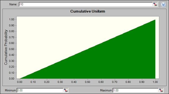
4. Another distribution, available in Crystal Ball, is that of the Uniform Distribution. If a Uniform Distribution is defined with Minimum = 0 and Maximum = 1.0, as shown below, then this distribution can be used to ascertain the underlying sequence of random numbers employed.

5. Excel provides the function BETADIST(Probability, Alpha, Min, Max) and if the sequence of numbers developed from the Uniform Distribution are fed into this equation, with the Alpha, Beta, Min and Max parameters set to the values above; namely Alpha = 2.78692, Beta = 9.12524 Min = 18.581 and Max = 760332
6. It was found that the sequence of numbers developed by the Beta Distribution functions in Crystal Ball, produced the same values as were found using the Excel Beta Distribution function (small differences in the Nth decimal place in a few cases), such that for practical purposes they could be regarded as the same.
7. A test was then carried out in which the parameters above were tested against the sorted results of the 10,000 iteration simulation. The AD statistic calculated was 0.205288 which is rounded to the value presented in Crystal Ball of 0.2053
8. From the above it is concluded that the formula employed in Crystal Ball mirror the equations available in Excel and that the method of calculating the Anderson Darling statistic can also be replicated in Excel.